Article Text

Abstract
OBJECTIVE To test the hypothesis that enthesophyte formation and osteophyte growth are positively associated and to look for associations between bone formation at different sites on the skeleton so that a simple measure of bone formation could be derived.
METHODS Visual examination of 337 adult skeletons. All common sites of either enthesophyte or osteophyte formation were inspected by a single observer who graded bone formation at these sites on a 0-3 scale. The total score for each feature was divided by the number of sites examined to derive an enthesophyte and an osteophyte score. Cronbach’s α and principal components analysis were used to identify groupings.
RESULTS Enthesophyte formation was associated with gender (M>F) and age. There was a positive correlation between enthesophytes and osteophytes (r = 0.65, 95% confidence interval, 0.58 to 0.71) which remained after correction for age and gender. Principal components analysis indicated four different groupings of enthesophyte formation. By choosing one site from each group a simple index of total skeletal bone formation could be derived.
CONCLUSIONS Osteophytes and enthesophytes are associated, such that a proportion of the population can be classified as “bone formers”. Enthesophyte groupings provide some clues to aetiopathogenesis. Bone formation should be investigated as a possible determinant of the heterogeneity of outcome and of treatment responses in common musculoskeletal disorders.
Statistics from Altmetric.com
Musculoskeletal disorders are associated with the formation of new bone at two main sites: the joint margin (osteophytosis) and ligament and tendon insertions (enthesophyte formation).1 ,2 Osteophytes are strongly associated with osteoarthritis, probably forming in response to abnormal stresses on the joint margin.3 However, the degree of osteophytosis in osteoarthritis varies considerably, and there is some evidence that small marginal osteophytes can also develop as an age related phenomenon, unrelated to any joint disease.4 New bone can form at individual entheses in response to a seronegative spondarthritis.5 More commonly, they are seen in several sites as part of the condition first described in the spine by Forrestier and Rotes-Querol6 and now known as diffuse idiopathic skeletal hyperostosis (DISH).7
The presence of periarticular osteophytes has been noted by Resnick and Niwayama in DISH1 but the relation of enthesophyte and marginal osteophytosis in this condition has not been specifically investigated. This study tests the hypothesis that some individuals have a greater tendency to form bone at both joint margins and entheses than others. The hypothesis has been derived from the observation in skeletal studies of striking osteophyte formation in a subgroup of skeletons, including those with DISH, and from the reports quoted above. The latter suggests that a variable amount of bone formation occurs at these two sites as a result of a mixture of age, a systemic predisposition, and local biomechanical factors.
Radiographs provide an insensitive and inadequate way of assessing osteophyte formation and enthesophyte changes.8 In contrast, the visual examination of skeletons allows all aspects of the joint margin and several different ligament and tendon insertion sites to be examined in detail, and graded for the amount of bony change. We have therefore systematically examined a number of skeletons for evidence of bony changes at several joint margins and enthesophyte sites, and examined the data for associations.
The unique opportunity of visual examination of whole skeletons also allowed us to document enough enthesis sites to investigate the data for possible groupings, which might provide insights into the aetiopathogenesis of enthesopathy as well as developing a method of quantifying the phenomenon and thus allowing us to derive a simple measure of “bone formation”. The development of a working definition is necessary before any clinical implications can be investigated.
Methods
Three hundred and thirty seven adult skeletons from routine studies of the skeletons from three separate archaeological sites were selected for entry into this project. All the data were collected according to our standard protocols and were acquired before deciding to use them to examine the hypothesis addressed in this paper. Each skeleton had at least half of all skeletal elements surviving, including the spine and the main long bones. Missing bones were assumed to be missing at random. There were 202 male skeletons, 129 female, and six were unsexed. The age ranges were young adult (20-25 years) to old adult (more than 60 years), as aged by standard anthropological techniques.9 ,10 The skeletons were dated from between the 9th century and the 16th century; 91 were from excavations at Wells Cathedral, 165 from St Oswald’s priory in Gloucester, and 81 from St Peter’s Church, Barton-on-Humber. All available skeletons from the sites at Wells and St Oswalds were used, and a further group from Barton-on-Humber was added to increase the power of the study. The skeletons were observed for osteophyte around the margins of vertebral bodies and at 23 peripheral joint sites, and enthesophyte at 14 ligament insertion sites (table 1). The joint sites were selected to include most synovial articulations around the skeleton. The odontoid peg was observed separately from the rest of the cervical facet joints. In the spine the presence of osteophyte at any cervical, thoracic, or lumbar facet joint was deemed to be positive for that segment. The three compartments of the knee joint were observed as individual joints and the thumb base was treated separately from the rest of the carpal-metacarpal joints. The presence of osteophyte in any metacarpal-phalangeal (MCP) joint, a proximal interphalangeal joint(PIP), or a distal interphalangeal joint counted as positive for that site. A similar regime was adopted for the foot. We selected a wide distribution of ligament insertion sites around the skeleton, mainly those noted by Resnick to produce enthesopathy in DISH. They were also sites where new bone formation at the enthesis was unequivocal. The osteophytes and enthesophytes were graded on a scale of 0-3 (none, mild, moderate, severe) (fig 1). The four point grading scales were adopted as being a usual way of grading osteophytes, for example, on x rays11 and have been adopted in palaeopathological studies so as to be as compatible with clinical work as possible. The presence or absence of DISH was also recorded according to criteria defined by Resnick.12
Osteophyte and enthesophyte locations

(A) Knees showing marked osteophytes grade III and enthesophytes at the tibial tubercle grade II. (B) Grade III osteophyte around the carpo-metacarpal joint of the thumb. (C) Calcaneum with grade II enthesophyte and patellae with grade III enthesophyte. (D) Radius with grade II enthesophyte at occipital protuberance and grade I osteophyte at radioulnar articulation. Ulna humeral joint has grade II osteophyte. (E) Hip joint showing greater trochanter of femur with grade II enthesophyte and lesser trochanter with grade I enthesophyte. The iliac crest also has enthesophytes, grade I, and the ischial tuberosity enthesophytes grade II.
STATISTICAL METHODS
An osteophyte score for each skeleton was obtained by adding all scores together and dividing by the number of joint sites for which observations could be made. Likewise enthesophyte scores were obtained by adding them together and dividing by the number of ligament insertion sites that were present for that individual. Thus the maximum osteophyte and enthesophyte scores for an individual was 3 for osteophyte and 3 for enthesophyte.
Both osteophyte and enthesophyte scores have been summarised with median scores and interquartile ranges. Spearman’s rank correlation was used to assess the strength of relations between continuous measures. Mann-Whitney tests were used to test for a difference in median scores between groups (for example, between sexes). A general linear model was used to assess the strength of the relations between enthesophyte scores and osteophyte scores while allowing for other potential confounding variables. A square root transformation was taken of the enthesophyte score (the dependent variable) in order to achieve normally distributed residuals. Statistical significance was set at the 5% level.
An attempt was made to find a small number of enthesophyte sites that could be used to construct an enthesophyte score with little loss of information (referred to as the reduced score). Cronbach’s α (a form of intraclass correlation coefficient) was used to identify sites that correlated poorly with others (that is, those sites which resulted in an increase in Cronbach’s α when omitted) in order to make an initial reduction in the number of sites used for scoring. Principal components analysis was used to identify possible “groupings” of enthesophyte sites with the intention of selecting sites to represent each grouping.
We have also considered different definitions of a “bone former” based on a dichotomy of the reduced score (that is, defining individuals as Bone formers or not, depending on whether their reduced score is above or below a particular cut off point). We have attempted to validate this by comparing our bone former definition with DISH as defined by Resnick and Niwayama.12
Results
Osteophyte and enthesophyte scores were calculable in all 337 skeletons. Both scores showed a positively skewed distribution (fig 2and 3). The median osteophyte score was 0.087, (interquartile range, 0 to 0.318). A total of 130 skeletons had a score of zero. The median enthesophyte score was 0.071, (interquartile range, 0 to 0.214). A total of 168 skeletons had a score of zero.

Histogram of the frequencies of skeletons in each category of osteophyte score. Each category has a range of 0.2 units. A positive skew is clearly evident

Histogram of the frequencies of skeletons in each category of enthesophyte score. Each category has a range of 0.2 units. A positive skew is clearly evident.
There was a strong positive correlation between osteophyte score and enthesophyte score (Spearman’s rank correlation, r = 0.647, 95% confidence limits = 0.579 and 0.706). The median enthesophyte score for males (0.080, interquartile range, 0 to 0.357) was significantly different (P < 0.001, Mann-Whitney test) from the median score for females (0, interquartile range, 0 to 0.100). Those in the older age group (> 45 years) had a higher median enthesophyte score (0.214, interquartile range, 0.071 to 0.538) than those in the younger age group (0, interquartile range, 0 to 0.083). This was also statistically significant (P < 0.001, Mann-Whitney test).
A general linear model using enthesophyte score as the dependent variable was constructed to test for a significant relation with osteophyte score whilst allowing for both sex and age effects. The parameter estimates for this model indicated a significantly higher enthesophyte score for males than for females (parameter estimate, males-females, = 0.079, SE = 0.026, P = 0.003) and also higher for the older age group (parameter estimate = 0.132, SE = 0.029, P < 0.001). In the presence of these effects there was also a significant osteophyte effect (parameter estimate = 0.679, SE = 0.051, partial correlation = 0.534, 95% confidence limits, 0.450 and 0.609).
The presence of DISH was identified in 28 individuals. The median enthesophyte score for these individuals was 0.667 (interquartile range, 0.432 to 0.893) compared to a median score of zero (interquartile range 0 to 0.167) in those without DISH. This difference was statistically significant (P < 0.001, Mann-Whitney test). The median osteophyte score for those with DISH was 0.711 (interquartile range 0.457 to 0.929) compared to a median score of 0.067 (interquartile range 0 to 0.222) for those without. This difference was also statistically significant (P < 0.001, Mann-Whitney test).
The overall value of Cronbach’s α (0.923) indicated a high degree of correlation between the enthesophyte scores at different ligament insertion sites. The omission of any single site resulted in very little change in Cronbach’s α. The lowest value (0.910) resulted from the omission of the iliac crest; the highest value (0.928) resulted from the omission of the rotator cuff. Cronbach’s α was therefore of little use in the selection of a reduced number of sites.
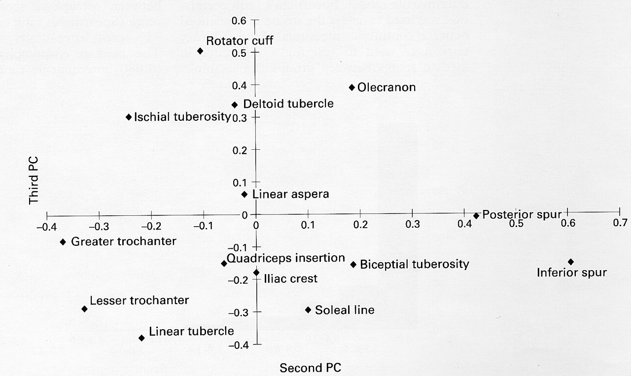
The principal components analysis resulted in three components which, combined, accounted for more than 68% of total variation. The first component (accounting for 53% of the total variation) contained positive coefficients from all sites and can be interpreted as a “size” component. The second (accounting for 8% of total variation) and the third (accounting for 7% of total variation) represent different modes of variation and were used to select four sites for consideration. These two components plotted against each other are shown in fig 4. Four groupings were identified: (1) the posterior and inferior spurs of the calcaneum; (2) the soleal line of the tibia, the bicipital tuberosity of the radius, the iliac crest, and the quadriceps insertion of the patella; (3) greater and lesser trochanters of the femur and the tubercle of the tibia; (4) the rotator cuff, olecranon process of the ulna, deltoid tubercule of the humerus, and ischial tuberosity of the pelvis. These groups are summarised in table 2. One ligament insertion site was arbitrarily chosen from each group. These four sites were the posterior spur of the calcaneum, the bicipital tuberosity of the radius, the greater trochanter of the femur, and the ischial tuberosity (see fig 1C-1E).

The loadings from each of the ligament insertion sites for the second and third principal components. This plot has been used to informally identify four groups of sites.
Four groups of ligament insertion sites
Based on these four sites, a reduced score (the average score of these four sites) was calculated. In one individual all four sites were missing and hence a score could not be calculated. In the remaining 336 the reduced score was compared with the full score and the differences examined. The mean difference was 0.011 (standard error = 0.0090); the standard deviation was 0.160. Therefore, assuming these errors follow a normal distribution, approximately 90% of the reduced scores would lie within the range (-0.252, 0.274) of the full score.
Possible definitions of a “bone former”were investigated using different dichotomies of this four-site reduced score. The sample prevalence of Bone formers was calculated for each definition together with percentage agreement (both sensitivity and specificity) with the presence or absence of DISH. These are shown graphically in fig 5. A definition based on a reduced score of greater than 0.30 agrees to a reasonable extent with the presence or absence of DISH (sensitivity = 78.6%, specificity = 83.2%) and would indicate a prevalence of Bone formers of approximately 22%.

Characteristics of different “bone former” definitions—agreement with occurrence of DISH and prevalence.
Discussion
The visual examination of skeletons provides a unique opportunity to describe bony changes related to age and disease. They allow all aspects of bony surfaces to be assessed, free of soft tissues. The commonest types of bony change seen in adult skeletons include osteophytes and enthesophyte formation.13 Osteophytes can be defined as lateral outgrowths of bone at the margin of the articular surface of a synovial joint. An enthesophyte is a bony spur forming at a ligament or tendon insertion into bone, growing in the direction of the natural pull of the ligament or tendon involved.
Both osteophyte and enthesophyte can be regarded as skeletal responses to stress. Osteophytes can occur as a part of the aging process but are more commonly associated with osteoarthritis. There is experimental evidence that osteophyte formation is related to instability of joints and their growth has been described as part of the attempt of a synovial joint to adapt to injury, limiting excess movement and helping to recreate a viable joint surface.14 Enthesophytes can form in response to the inflammation of the enthesis occurring in seronegative spondarthropathies and in response to repetitive strain, as in the spiking of tibial spines seen in footballers.15Enthesophyte formation also occurs in the absence of any clear cause. Multiple idiopathic enthesophytes are characteristic of diffuse idiopathic skeletal hyperostosis (DISH).7
The hypothesis that there may be a relation between marginal osteophytes and enthesophytes has been alluded to by Resnick1 and was suggested to us by the observation of skeletons with excessive bone formation of both types, with or without DISH. However, this is the first systematic study to examine this hypothesis. A biological rationale might be that the response of the skeleton to stress depends on common cellular mechanisms, which site is affected, and the genetic control of the reaction.
To address this hypothesis, multiple sites prone to either osteophyte or enthesophyte formation were examined in a large number of skeletons. The data were collected by a single experienced observer, able to grade the severity of bone formation at different sites, as well as the presence or absence of change. It is possible that due to a lack of blinding the observation of one change may have influenced the recording of the other. We think this is unlikely to have been of importance, however, because the data were collected before the hypothesis developed and because the changes are so clear on skeletons. The data shows a similar distribution of each type of bony growth: these “Bone formers” forming a substantial minority of the skeletal population. As expected,2 enthesophyte formation was associated with age and was more common in males than females.
The major finding of the study was the strong positive relation between enthesophytes and osteophytes. The data were analysed carefully to exclude the possibility of this being due to age and sex associations alone. The validity of the association was reinforced by the finding that skeletons with the most extensive enthesophyte formation (that is, those with DISH) also had very high osteophyte scores.
Enthesophytes, when present, were frequently seen in many sites. The data were examined, therefore, to look for patterns or groupings. Using Cronbach’s α, a strong association between all sites was suggested, but no obvious groups emerged. However, a principal components analysis indicated a possible division into four groups of sites which were more strongly associated with each other. The grouping, together of the two calcaneal sites in one group and the two femoral trochanters with the tibial tubercle in another, suggests that local biomechanical factors may lie behind these groupings. However, the two other groupings link upper and lower limb sites, perhaps indicating that systemic factors such as body habitus may also be important. In this context DISH is known to be associated with both diabetes and obesity.16 ,17
By using one site from each grouping, a simple assessment of overall skeletal bone formation was derived, which was a reasonable approximation of the total enthesophyte score. This could allow skeletons to be assessed quickly and easily. It also implies that a few simple radiographs could be used to provide an assessment of bone formation in vivo.
Bone formation is one of the major components of the response of the musculoskeletal system to stress and injury, as evidenced by Wolff’s law of bone remodelling. This study suggests that the observed variation in bone formation could be due to differences in individual ability to form bone in response to stress rather than differences in stress. This suggests a heterogeneity in one of the fundamental aspects of the pathogenesis of musculoskeletal disorders which may be under genetic control. Individuals who are good bone formers may have different disease outcomes to those of poor bone formers. Our findings indicate that simple indices of bone formation can be derived from skeletons and these may be generalisable to radiographic examinations. The concept of bone formers should now be examined in relation to the heterogeneity of outcome and treatment responses in disorders such as osteoarthritis and osteoporosis.